Butterfly Networks
This is about the butterfly network topology. We’ll walk through how it naturally arises in the FFT algorithm. Then I’ll discuss some nice properties and use cases for butterfly networks.
Topics
Motivation (polynomial multiplication)
Consider the problem of multiplying two polynomials
\[\\ a(x)=\sum_{i=0}^d a_ix^i; b(x)=\sum_{i=0}^d b_ix^i \\\]. The degree of $a,b$ is just $d$ – the largest power of $x$ appearing in the polynomials. In middle school, we learn a simple $O(n^2 )$ double-summation approach to multiplying these:
\[\\ C(x)=a(x)b(x)=\sum_{i=0}^d \sum_{j=0}^d a_ib_jx^{i+j} \\\]We’ll try to improve to $O(n \log n)$ time. Assume for simplicity that $n=d+1$ is a power of 2. Let’s consider how we are representing the polynomials $a,b$. We’re currently specifying $a$ via its coefficient representation $[a_0,…,a_d]$; likewise for $b$.
As an alternative specification, suppose we are given a selection of distinct points, $x_1,…,x_n$, at which $a(x),b(x)$ are evaluated. From algebra, we know that a polynomial can also be fully specified by its values $n$ distinct points. Hence, we can also fully specify $a$ via its evaluation representation $[a(x_1 ),…,a(x_n )]$.
How does this help us? If we know $a(x_1 ),b(x_1)$, clearly we also know $C(x_1)$ by simply multiplying $a(x_1) \cdot b(x_1)$. So if we manage to convert $a,b$ from coefficient representation to evaluation representation, we can quickly compute $C$’s evaluation representation. Then, if we can convert the other way around – from $C$’s evaluation representation to $C$’s coefficient representation – we’re done!
That’s exactly what we’ll try to do below. In particular, we’ll focus on converting $a$ from coefficient representation to evaluation representation. This conversion is called a Discrete Fourier Transform (DFT), and the Fast Fourier Transform (FFT) is an algorithm to do the conversion quickly. (The reverse conversion, and Inverse DFT, uses similar ideas, so we won’t discuss it here.)
This example is based on these great lecture notes and this video.
Fast Fourier Transform
Let’s take a divide and conquer approach. Write a degree-$d$ polynomial as the sum of two $\approx d/2$ degree polynomials. We can do this by grouping even and odd terms together.
\[\\ a(x)=[a_0+a_2 x^2+\cdots+a_{d-1} x^{d-1} ] \\\] \[\\ +x[a_1+a_3 x^2+\cdots+a_d x^{d-1} ] \\\]Notice how we pulled the $x$ out of the odd group, so that now each group only has even terms. This allows us to write a simple decomposition:
$a(x)=a_+ (x^2 )+xa_- (x^2 )$, where
Then, in the spirit of divide and conquer, we further divide each of $a_+,a_-$, to get four polynomials, each of degree $\approx d/4$. We’ll divide $a_+$ into $a_{++}, a_{+-}$, and we’ll divide $a_-$ into $a_{-+}, a_{–}$.
For instance, $a_{++}$ will contain the coefficients $a_i$ where $i$ is a multiple of 4; and $a_{-+}$ will contain $a_i$ where $i$ is 3 greater than a multiple of 4. We can keep doing this until each of our small polynomials consists of just one constant term $a_j$.
How long will it take? Well, all we’ve done here is just turned a degree-$d$ polynomial into $d+1$ degree-1 polynomials. Evaluating a single $a(x_i)$ will still take $O(n)$ time, so evaluating $a(x_1 ),…,a(x_n)$ still takes $O(n^2 )$ time. We’ll have to make further improvements, which we can do by carefully choosing the $x_1,…,x_n$.
Our goal in choosing these is to allow for reuse of polynomial evaluations. Consider $a_+ (x^2 )$ and $a_- (x^2 )$. If we choose $x_1=1,x_2=-1$, then $x_1^2=x_2^2$ and $a_+ (x_1^2 )=a_+ (x_2^2 )$. This means we can reuse the evaluation $a_+(1)$. As one guideline, for every $x_i$, we should also choose $-x_i$ to be in our set of points. Also apparent from above: we can save an evaluation if both $x_i$ and $x_i^2$ are in our set of points.
One particular set of numbers full of these desirable properties is the $n^{th}$ roots of unity; that is, the complex numbers $z_1,…,z_n$ satisfying $z_i^n=1$. The first root of unity is 1. The second roots of unity are 1,-1. The fourth roots of unity are $1,i,-1,-i$. In general, the roots of unity are just $n$ equally spaced points on the complex unit circle, starting with 1, as illustrated in Fig 1.
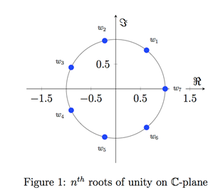
Figure 1 - 7th roots of unity on complex plane
Using these numbers makes it very easy to share sub-polynomial evaluations. For instance, as discussed above, in the n=4 case with $x_1=1,x_2=i,x_3=-1,x_4=-i$, we have
\[\\ a(n)=a_0+a_1 x+a_2 x^2+a_3 x^3 \\\] \[\\ =a_+ (x^2 )+xa_- (x^2 ) \\\]Note that $i^2= (-i)^2=-1$ and $-1^2=1^2=1$. This makes things easier, since
$a_+ (x_1^2 )=a_+ (x_3^2 )$; $a_+ (x_2^2 )=a_+ (x_4^2)$; $x_1 a_- (x_1^2 )=-x_3 a_- (x_3^2 )$, etc.
A single evaluation $a(x_i )$ requires traversing a complete binary tree of sub-polynomials. Likewise, evaluating $a(x_1),…,a(x_n)$ involves traversing $n$ of these complete binary trees. But the trees share nodes, and sometimes entire subtrees, in such a way that the entire transform can be computed in $O(n \log n)$ time, which is fast. This concept is illustrated in the next section.
Butterfly network topology
Let’s take a closer look at these trees of polynomials. Each arrow in the diagram is a (direct) dependency. For instance, the vertical uppermost red arrow indicates that computing $a(i)$ requires first computing $a_+ (-1)$ and $a_- (-1)$. To fully evaluate $a(x_2)$, we only require the connections outlined in red. To fully evaluate all points, $a(x_1),…,a(x_n)$, we require all of the red and blue connections. These connections form what’s called a butterfly network, simply because the two-node version looks like a butterfly. In Fig 2, you can see a butterfly at the bottom left, and another at the bottom right.
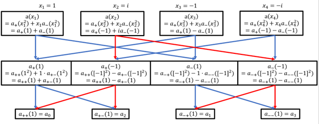
Figure 2: Butterfly Network for n = 4 FFT
In theory, FFTs are trivial to parallelize. To compute an FFT with input size $n$ on $p$ processors, you can start by having each processor evaluate $n/2^0 p$ of the degree-1 polynomials (the leaves of the tree shown above). Next, you can have each processor evaluate $n/2^1 p$ of the degree-2 polynomials, accessing the degree-1 solutions as needed, and continuing up the network. This is the natural approach to parallelizing any divide and conquer algorithm.
In practice, FFTs are often performed on huge images or complex audio signals, and the communication cost (i.e. transferring the stored solutions between processors) becomes prohibitively large. One obvious (but very involved) solution is to design your processor network in a way that reduces these costs. And in this case, the FFT algorithm readily illustrates its own ideal network topology. In Fig 2, the four boxes on top (the $x_i$ to be evaluated) represent processors, and the other 8 boxes represent routers or switching nodes. And of course, the arrows represent wires.
FFTs are important in computing – important enough that if necessary, butterfly networks would surely be built for the sole purpose of computing FFTs. As it turns out, the butterfly topology has nice properties that make it useful in other settings as well.
Properties and Applications
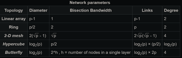
Figure 3 - Butterfly network performance evaluation compared to other network topologies.
- A network’s diameter is the max number of switches between any two processors. In Fig 2, going from P1 (processor 1) to P3 takes requires passing through just 1 router. P1 to P2 passes through 3 routers, as does P1 to P4. In general, a butterfly network requires passing through no more than $O(\log n) $ routers.
- A network’s bandwidth measures how many wires can be used before a bottleneck becomes inevitable. Butterfly networks have an extremely high bandwidth, as seen above.
- This speed and capacity comes at a cost. Butterfly networks are expensive to build, requiring more wires and routers than other network topologies.
In the polynomial example, we assumed that $n$ was a power of two. In their FFT algorithm, Cookey and Tukey made a similar assumption. Several years before that, in 1958, Good and Thomas suggested a prime-factor FFT algorithm which worked only for prime factors. Different FFT algorithms have emerged, and have been combined in different ways to support arbitrary n. One of the most popular libraries for FFT computation, FFTW, reflects this combined approach, but still runs more slowly if $n$ has fewer factors. FFTW also contains OpenMP and MPI implementations, as well as optimizations for special cases of the FFT.
FFT applications can be demanding, and oftentimes these optimizations are not sufficient. FFTs are often used to approximate a function as a sum of waves (sines and cosines) of varying frequencies, phases, and amplitudes. As Gauss discovered, some PDEs are more easily solved in frequency space. When transforming a function into frequency space, high $n$ can be used to achieve arbitrarily small approximation error, and thus more precise PDE solutions.
In communications, we often receive an audio signal in time space, and we want to know which frequencies (i.e. which waves) that signal is composed of. This can be useful in signal interpretation and denoising. For example, by filtering out waves outside the frequency of human voice, we can amplify the important signal and make it easier to hear speech. Once again, higher $n$ corresponds to a more thorough decomposition. Granted, the max $n$ you should use is limited by the audio sampling rate. A similar principle applies to images. As image definition and audio sampling rate increase, increasingly large FFTs are required to compress and denoise these media.
As a result, sometimes even the FFT is not fast enough, and we need other solutions like the sparse FFT. This is still an active area of research. Sparse FFTs can be used for sparse data – for instance, when a signal to contains just a small set of frequencies.
In high performance computing, scaling and hardware optimization are the most active areas of development. The FFT has already greatly benefitted from hardware optimization, including butterfly topologies to perform FFTs and image convolutions. But this remains a specialized topology, and many supercomputers including Summit and Fugaku are built for more general use cases. On these machines, communication remains costly, and sidestepping this bottleneck is an ongoing effort.