This post is about a cool way to speed up an $O(n^2)$ algorithm to $O(n\log n)$ runtime using annotated trees. 15 minute read if you’re familiar with binary trees, arrays, and big O notation.

Topics

Problem Formulation
Checking whether 2 chords intersect
Slow $O(n^2)$ Algorithm
Counting higher-numbered “open” chords
Annotated complete binary tree
Fast $O(n\log n)$ Algorithm

Problem Formulation

Let’s draw a few chords on a circle. A point on the circle’s circumference is identified by its polar angle $0^{\circ}\leq \theta < 360^{\circ}$, indicating the point’s counterclockwise angle from the green dashed line in Fig 1. A chord has 2 endpoints, each a point on the circle’s circumference. Thus, we will identify a chord using a tuple of its endpoint angles: $C_i = (s_i, e_i)$.

As input we are given $n$ chords, $C=[(s_0,e_0),…,(s_{n-1},e_{n-1})]$. For simplicity, assume no endpoints are reused (see Fig 1). We’ll discuss how to efficiently count the number $I$ of distinct pairs of intersecting chords.

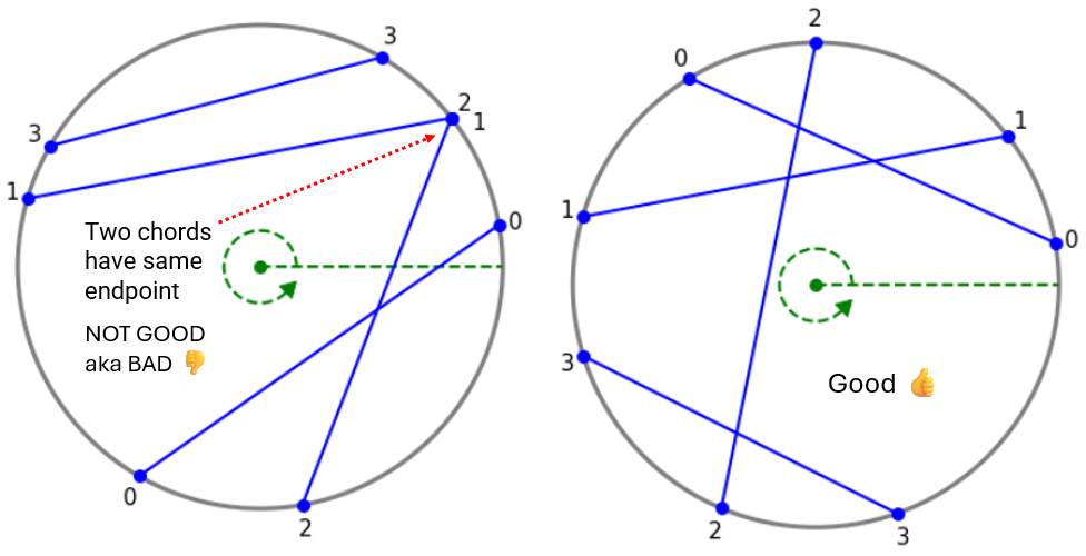
Figure 1 - No shared endpoints

Chord labeling procedure

Note that a chord doesn’t change if the starting and ending angles are swapped. $(s_i,e_i)$ is the same chord as $(e_i,s_i)$. Thus we can safely assume that $s_i<e_i$ (if not, then just go ahead and swap them). This is a preprocessing of $C$, and let’s call the preprocessed list $C’$.

As another preprocessing step, sort $C’$ in increasing order of starting angle $s_i$. We’ll call the sorted list $C”$. After this sorting, each chord’s label is its position in $C”$. Visually, starting at the green dashed line and proceeding counterclockwise, the chords are numerically labeled in the order of endpoint encounters. See the example below for clarity.

Example

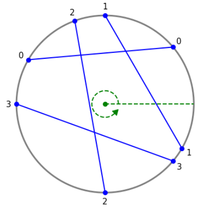
Figure 2 - Labeling the chords (gif)

Fig 2 shows $n=4$ chords labeled 0 thru 3. There are ${4\choose 2} = 6$ pairs of distinct chords. $I=4$ of these pairs intersect: 0 & 1, 0 & 2, 1 & 2, and 2 & 3. Chords 0 & 3 and 1 & 3 do not intersect.

Unprocessed input: $C = [(110^{\circ},270^{\circ}),(320^{\circ},180^{\circ}),$ $(90^{\circ},330^{\circ}),(150^{\circ},40^{\circ})]$

After sorting each tuple: $C’ = [(110^{\circ},270^{\circ}),(180^{\circ},320^{\circ}),$ $(90^{\circ},330^{\circ}),(40^{\circ},150^{\circ})]$

After sorting list: $C” = [(40^{\circ},150^{\circ}),(90^{\circ},330^{\circ}),$ $(110^{\circ},270^{\circ}),(180^{\circ},320^{\circ})]$.
The order of $C”$ gives the numeric chord labeling.

Number of possible intersections

Suppose each chord intersects each other chord. Then, as an upper bound, we have ${n\choose 2} = n(n-1)/2 = O(n^2)$ intersections. This suggests a simple $O(n^2)$ solution. Starting with $I=0$, check each pair of chords, and increment $I$ if they intersect.

How can we determine whether chords $C_i”=(s_i,e_i)$ and $C_j”=(s_j,e_j)$ intersect, for $i<j$?

Checking whether 2 chords intersect

Remember that we sorted $C”$ by starting angle. So if $i<j$, then $s_i$ must be the minimum of $s_i,e_i,s_j,e_j$. From here, convince yourself that there are only 3 possible orderings: $s_i<s_j<e_i<e_j$, or $s_i<s_j<e_j<e_i$, or $s_i<e_i<s_j<e_j$. Of these orderings, as illustrated in Fig 3, only $s_i<s_j<e_i<e_j$ indicates an intersection between chords $i$ and $j$.

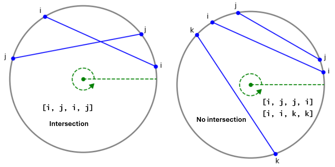
Figure 3 - Checking whether 2 chords intersect

Slow $O(n^2)$ Algorithm

Using this observation, we can write an $O(n^2)$ algorithm which just checks each pair of chords for an intersection:

Algorithm 1 - slow intersection counting

Input: $C=[(s_0,e_0),…,(s_{n-1},e_{n-1})]$, where $s_k,e_k$ are endpoint angles of chord $k$.
Output: $I$, the number of intersecting pairs of the given chords.

Initialize $I=0$
for $k=0,n-1$:
if $s_k>e_k$ then swap$(s_k,e_k)$
$C”$ = $C$ sorted by increasing $s_k$

for $i=0,n-1$ do
Get chord endpoints $(s_i,e_i)$ $=C”[i]$
for $j=i+1,n-1$ do
Get chord endpoints $(s_j,e_j)$ $=C”[j]$
if $s_i<s_j<e_i<e_j$ then
increment $I$

The sorting step takes $O(n\log n)$ time, and the nested for loops take $O(n^2)$ time. Next we’ll describe a faster algorithm.

Sorted list of endpoint labels

Starting with $C”$, construct a new list $P$ as follows: for every $(s_i,e_i)$ in $C$, add $(s_i,i)$ and $(e_i,i)$ to $P$. Each entry in $P$ contains the angle of an endpoint, and the numeric label of that endpoint.

Now sort $P$ by increasing angle to get $P’$. For Fig 2’s example, $P’$ is $[(40^{\circ},0),(90^{\circ},1),(110^{\circ},2),(150^{\circ},0),$ $(180^{\circ},3),(270^{\circ},2),(320^{\circ},3),(330^{\circ},1)]$. As a final step, completely remove the angles, such that $P”$ is just a list of $2n$ endpoint labels in their order of appearance, e.g. $P”=[0,1,2,0,3,2,3,1]$.

Counting higher-numbered “open” chords

We’ll try counting intersections via a single loop thru $P”$. As we loop through $P”$, let’s call a chord “open” if we’ve encountered exactly one of its endpoints, and “closed” if we’ve encountered neither or both of its endpoints.

Refer to Fig 4. During our loop, first we come across chord 0, then chord 1, then chord 2 - all three of these chords are now open. Then we come across chord 0 again. This means the endpoints of chords 0 and 1 occur in the sequence $[0,1,0,1]$, as in Fig 3’s left diagram. Therefore, chord 0 intersects chord 1. Likewise for chords 0 and 2. Every time we close chord $i$, if we know how many higher-numbered chords are open, say $o_i$, then there are simply $I=o_1+\cdots+o_n$ total intersections.

Figure 4 - Slow algorithm illustration (click arrow to fast forward)

The “higher-numbered” condition is crucial. Without it, we would count a false intersection between Chords 1 & 2, since 1 is still open when we close 2. With this method, checking each open chord takes $O(n)$ time (worst case). Clearly, doing so each time we close a chord just produces another $O(n^2)$ algorithm. Can we do better? In particular, when we close a chord, can we count how many higher-numbered chords are currently open in less than $O(n)$ time?

Indexed complete binary tree

It turns out we can’t do better. Just kidding, we can. We’ll count higher-numbered chords in $O(\log n)$ time by extending a complete binary tree. For those interested, this is similar to the Rank function for order statistic trees.

Our tree $T$ will have one leaf node for each of the $n$ chords. All leaf nodes reside at the same depth level, $d=\lceil \log n \rceil$, where the root has depth 0. (Logs in this post use base 2.)

The leafs have the same left-to-right order as the numeric chord labelings. For instance, Chord 0 corresponds to $T$’s leftmost leaf, and Chord $n-1$ corresponds to the rightmost leaf. Since we know $n$’s value, we can construct $T$ by adding leafs one at a time. Each leaf addition takes $d=O(\log n)$ time, so constructing $T$ with $n$ leafs takes $O(n\log n)$ time.

For quick constant-time access to leafs (indexing), we can use a leaf array $LF$ with $LF[i]$ pointing to Chord $i$’s leaf node in $T$. This isn’t necessary, but will make life easier. And to quickly navigate $T$, each node has 3 pointers: left child, right child, and parent.

Annotating the tree

Each tree node, leaf or not, is annotated with a “size”. Leaf $i$’s size is 1 if Chord $i$ is open, 0 otherwise. A non-leaf’s size is the number of open leafs in its subtree. For instance, the root’s size is equal to the total number of open leafs. Before looping thru $P”$, all nodes have initial size 0.

What happens when we open chord $i$? Clearly, we should set $LF[i]$’s size to 1. Each of $i$’s ancestors’ sizes should also be incremented, since one leaf in their subtree was newly opened. This takes $O(\log n)$ time. Likewise, closing chord $i$ requires setting $LF[i]$’s size to 0, and decrementing each of $i$’s ancestors’ sizes.

Now, back to the reason we created $T$: When we close a chord, we need to quickly count how many higher-numbered chords are still open.

Suppose node $R$ is a right child of its immediate parent $A$. Consider the highest-numbered leaf $B$ in the subtree rooted at $A$. Since the leafs are in increasing order from left to right, $B$ must also be in the subtree rooted at $R$. Thus, $A$ contains no higher-numbered leafs than $R$.
Suppose node $L$ is a left child of $A$, and $A$ has right child $R$. Then every single open leaf in the subtree rooted at $R$ is higher-numbered than any leaf in the subtree rooted at $L$. Again, this follows from the left-to-right ordering of the leafs in the tree.

This gives a recursive $O(\log n)$ procedure for counting how many higher-numbered chords are open when we close Chord $i$. See Fig 5 for an illustration.

Algorithm 2 - recursively count higher-numbered leafs

Input:
Complete binary annotated tree $T$
Numeric chord label $i$ to close
$LF$, array of pointers to leafs of $T$
Output: Number $G$ of currently open chords with numeric label $>i$

Initialize $G=0$, cur $= LF[i]$
while cur’s parent isn’t null:
set A to cur’s parent
if cur is left child of A then
add size of A’s right child to $G$
set cur to A

Final $O(n\log n)$ algo

Figure 5 - Fast algorithm illustration (click arrow to fast forward)

Now that we can count a single chord’s higher-numbered intersections in $O(\log n)$ time, we can do this for each chord to get an $O(n\log n)$ algorithm. Illustration in Fig 5, pseudocode below.

Algorithm 3 - fast intersection counting

Input: $C=[(s_0,e_0),…,(s_{n-1},e_{n-1})]$, where $s_k,e_k$ are endpoint angles of chord $k$.
Output: $I$, the number of intersecting pairs of the given chords.

Initialize intersection count $I=0$
Initialize $n=$ length$(C)$
Initialize complete binary tree $T=$ root node
Any node added to $T$ starts with size = 0
Initialize depth $d=\lceil \log n \rceil$
Initialize array $LF$ of length $n$

for $k=0,n-1$ do
Add a leaf to $T$ at depth $d$
Leaf should be as far left as possible
Set $LF[k]$ to point to the leaf
Compute $P”$, an array of $2n$ chord labels
(this is the preprocessing of $C$ described above)
for $i=0,2n-1$ do
Get next chord label $m=P”[i]$
if $LF[m]$ is 0 then
Increment the leaf’s and its ancestors’ sizes
if $LF[m]$ is 1 then
Set $G=$ higher-numbered leaf count (Algorithm 2)
Decrement the leaf’s and its ancestors’ sizes
Update total intersection count: $I=I+G$