Gibbs Sampling and Hierarchical Bayes
We’ll give an overview of Gibbs sampling here, and point to some basic research regarding its practical use. Some background in probability is assumed.
History of the term
In 1868, while studying thermal properties of gases, physicist Ludwig Boltzmann discovered a probability distribution describing the state of a system of particles as a function of the system’s energy and temperature. This distribution was further studied by physicist Josiah Gibbs in 1902, and today it’s called the Gibbs distribution or the Boltzmann distribution.
Fast forward to 1984, when the German brothers and Stuart German (UMass Amherst) developed an algorithm with roots in statistical mechanics to recover degraded images. This algorithm required sampling from the Gibbs distribution, and to achieve this, the German brothers developed and proved convergence of a sampling method which they coined the Gibbs sampler. While similar methods may have been used earlier, the Gibbs sampler was popularized by this paper, so the name stuck. Today, that paper remains fundamental and highly cited, and the Gibbs sampler is used more frequently than ever.
Description of Gibbs Sampling
Motivation: sampling from a joint distribution
Suppose we have 2 random variables $X,Y$ with joint probability distribution
\[\\ k_{X,Y}(x,y) \sim N\left( \begin{bmatrix} 0 \\ 0 \end{bmatrix},\begin{bmatrix} 1 & 0.5 \\ 0.5 & 1 \end{bmatrix} \right) \\\]which is the standard bivariate normal distribution with correlation coefficient $ \rho = \frac{1}{2} $.
Now let $ W(x,y) = xy\sqrt{\log{(x + y)}} $. How do we compute $E\left\lbrack W(X,Y) \right\rbrack$?
As a first attempt, we can use the law of the unconscious statistician:
\[\\ E\left\lbrack W(X,Y) \right\rbrack = \int_{- \infty}^{\infty}{\int_{- \infty}^{\infty}{k(x,y)W(x,y)} dx dy} \\\] \[\\ = \int_{- \infty}^{\infty}{\int_{- \infty}^{\infty}\frac{xy\sqrt{\log{(x + y)}}}{2\pi\sqrt{0.75}}\exp\left\lbrack - 2(x^{2} - xy + y^{2}) \right\rbrack dx dy} \\\]As we can see, this gets very messy. This density does not match that of any well-studied bivariate distribution, and even Wolfram times out when trying to compute it in closed form.
Let’s take a different route, and instead try simulating this integral. First, we draw a sample $\lbrack\left( X_{1},Y_{1} \right),\ldots,\left( X_{n},Y_{n} \right)\rbrack$ of size $n$ from $k_{X,Y}$, which is just a set of pairs $(X_{i},Y_{i})$ with $k_{X,Y}\left( x_{i},y_{i} \right) > 0$. Ideally, these pairs should be selected such that the probability of observing a pair $(X_{i},Y_{i})$ in the sample is proportional to that pair’s joint density $k_{X,Y}\left( x_{i},y_{i} \right)$.
Clearly, once we have selected the sample, it is easy to estimate $E\left\lbrack W(X,Y) \right\rbrack$ by computing $W\left( X_{i},Y_{i} \right)$ for each draw in the sample, and averaging those results:
\[\\ E\left\lbrack W(X,Y) \right\rbrack \approx \frac{1}{n}\sum_{i = 1}^{n}{W\left( X_{i},Y_{i} \right)} = \frac{1}{n}\sum_{i = 1}^{n}{x_{i}y_{i}\sqrt{\log{(x_{i} + y_{i})}}} \\\]From this example, it should be clear why sampling from a joint distribution can be useful.
Example Gibbs sampling procedure
But how do we select the sample to begin with? In the univariate case, we can sample from a distribution directly by passing $Unif(0,1)$ samples through that distribution’s inverse CDF. In the bivariate case, however, the inverse CDF would be a bijection from $\lbrack 0,1\rbrack \rightarrow R^{2}$, which may not exist.
Fortunately, we have tools available for sampling from bivariate normal distributions. One method, described by Rasmussen & Williams in their book GPML, involves computing a Cholesky decomposition and sampling twice (since this is a bivariate joint distribution) from the univariate standard normal distribution. Let’s devise an alternative method – one involving less linear algebra – for sampling from $k_{X,Y}$.
We know that the conditional distributions of a bivariate normal are each univariate normal:
$g_{Y|X}\left( y \vert X = x \right) \sim N\left( \rho x,1 - \rho^{2} \right)$ and $g_{X|Y}\left( x \vert Y = y \right) \sim N\left( \rho y,1 - \rho^{2} \right)$.
Thus, given an $x_{1}$, we can then sample $y_{1}$ from $g_{Y|X}\left( y \vert X = x_{1} \right)$, and together the pair $(x_{1},y_{1})$ will form a draw from $k_{X,Y}$, which was our stated goal. And this argument is symmetrical in $x$ and $y$; we could also start with $y_{1}$ and sample from $g_{X|Y}\left( x \vert Y = y_{1} \right)$. Thus, we have the following procedure for sampling from $k_{X,Y}$, i.e. for generating $\lbrack\left( X_{1},Y_{1} \right),\ldots,\left( X_{n},Y_{n} \right)\rbrack$:
(1) Choose $x_{1} \in R$, and set $i = 1$.
(2) Sample $y_{i}$ from $N\left( \rho x_{i},1 - \rho^{2} \right)$.
(3) Record $(x_{i},y_{i})$, and increment $i$.
(4) Sample $x_{i}$ from $N\left( \rho y_{i - 1},1 - \rho^{2} \right)$.
(5) If $i \leq n$, then cycle back to step (2).
At the end, we have a sample $\lbrack\left( X_{1},Y_{1} \right),\ldots,\left( X_{n},Y_{n} \right)\rbrack$ from the joint distribution $k_{X,Y}$. This is Gibbs sampling!
Intuition
Let’s reflect on what we just did. To estimate a difficult-to-compute expectation, we wanted to sample from a bivariate normal distribution $k_{X,Y}(x,y)$, which is pictured in Figure 1. But we ran into a problem: it was also difficult to sample from $k_{X,Y}(x,y)$ directly. However, we observed that the conditional distributions $g_{Y|X}$ and $g_{Y|X}$ were both univariate normal, and were easy to sample from.
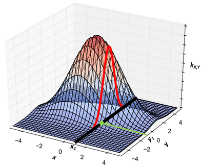
So we chose a starting value $x_{1}$ (We didn’t specify how that starting value was chosen – we’ll discuss that later.) Then we computed the conditional probability of $y$ given $x_{1}$. For instance, $g_{Y|X}\left( y \vert X = x_{1} \right)$ is the univariate normal distribution shown by the red line in Figure 1. We then sampled $y_{1}$ from that conditional, thus establishing $(x_{1},y_{1})$ (indicated by the green dot) as our first draw from $k_{X,Y}$.
The joint distribution is pictured from a different angle in Figure 2, with the green dot still representing $(x_{1},y_{1})$. Note that the green dot’s horizontal position in Figure 2 was already established by our initial choice $x_{1}$, and its vertical position $y_{1}$ was established by sampling from $g_{Y|X}\left( y \vert X = x_{1} \right)$. To compute our second draw $(x_{2},y_{2})$, we first take a horizontal step by sampling from $g_{X|Y}\left( x \vert Y = y_{1} \right)$. Then we take a vertical step by sampling from $g_{Y|X}\left( y \vert X = x_{2} \right)$. Following the black arrows, we now have $(x_{2},y_{2})$ as our next draw from $k_{X,Y}$!
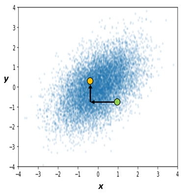
Intuitively, what’s happening is we’re selecting an initial x-coordinate. From there, each conditional draw from $g_{Y|X}$ is nudging us up or down, with a bias to move toward higher-probability regions of the conditional. Likewise, each conditional draw from $g_{X|Y}$ nudges us left or right. We are more likely to move toward higher-density regions of $k_{X,Y}$, but sometimes we might get a surprising draw that pushes us to a lower-density point. For this reason, we consider $\lbrack\left( X_{1},Y_{1} \right),\ldots,\left( X_{n},Y_{n} \right)\rbrack$ to be a random sample from $k_{X,Y}$. In fact, under reasonable conditions detailed by Roberts & Smith in this paper, as $n \rightarrow \infty$ it is guaranteed that
\[\\ \frac{1}{n}\sum_{i = 1}^{n}{W\left( X_{i},Y_{i} \right)} \rightarrow \int_{- \infty}^{\infty}{\int_{- \infty}^{\infty}{k(x,y)W(x,y)}dx\ dy} \\\]The speed of convergence depends on the sampler’s mixing time, which is a term describing how large an $n$ is required for the sample’s distribution to approach the true joint distribution $k$.
Definition
Rather than just $X,Y$, let’s generalize to more than 2 variables. Call them $X^{(1)},\ldots,X^{(m)}$, with joint pdf $k\left( x^{(1)},\ldots,x^{(m)} \right)$, joint sample space $\Omega$, and conditionals $g_{j}\left( x^{(j)} \vert x^{(l \neq j)} \right)$. As before, suppose we cannot sample from $k$, but we can sample from each of the conditioanls $g_{1},\ldots,g_{m}$. In this case, Gibbs sampling is the following procedure, which generates $\left\lbrack \mathbf{X_1},\ldots,\mathbf{X_n} \right\rbrack$, where $\mathbf{X_i}\mathbf{=}\left( X_{i}^{(1)},\ldots,X_{i}^{(m)} \right),$ as our sample from $k$.
(1) Choose $\mathbf{x_1}\mathbf{\in}\Omega$, and set $i = 2$.
(2) For $j \in \lbrack 1..m\rbrack$:
Sample $x_{i}^{(j)}$ from $g_{j}\left( x^{(j)} \vert x_{i}^{(1)},\ldots,x_{i}^{(j - 1)},x_{i - 1}^{(j + 1)},\ldots,x_{i - 1}^{(m)} \right)$
(3) Record $\mathbf{x_i}\mathbf{=}\left( x_{i}^{(1)},\ldots,x_{i}^{(m)} \right)$, and increment $i$.
(4) If $i \leq n$, then cycle back to step (2).
This is very similar to our 2 variable procedure. One difference is that here, we are first fixing $\mathbf{x_1}$ as a full draw from the joint distribution. In contrast, for our 2 variable case, we only required choosing $x_{1}$ (as opposed to $(x_{1},y_{1})$), and we did one preliminary conditional sample to choose $y_{1}$. This difference is unimportant, as we will soon see. The important thing to note is that each conditional draw in Step (2) conditions on the most recent value of each $x^{(l \neq j)}$. If $x_{i}^{(l)}$ has already been computed, then we use it; otherwise, we resort to using $x_{i - 1}^{(l)}$.
Application: Hierarchical Bayes
g
Consider the problem of estimating the distribution of a parameter $\theta$. Suppose we have a prior belief that $\theta \sim h(\theta)$. Then, we observe data $x$ with likelihood $f(x \vert \theta)$. Applying Bayes’ theorem, we obtain a posterior distribution
\[\\ k\left( \theta \vert \mathbf{x} \right) \propto h(\theta)f(x|\theta) \\\]which describes our belief about $\theta$’s distribution after observing $x$.
Let’s think about how we might justify using such a model, including justifying our choice of $h(\theta)$. Say we’re heading to a new fishing spot, and we want to estimate $\theta$, the number of fish we’ll catch in an hourlong fishing session. Given our skill level, the weather, the time of year, and the nature of the spot, there should be some true mean rate of fish caught. And given that rate, how long it takes to catch one fish shouldn’t affect the time it takes to catch the next fish. Thus, even without prior data, it seems reasonable to say that $X \sim Poisson(\theta)$.
But what do we think the rate $\theta$ is, before actually fishing? We need a prior distribution $h(\theta)$, and in many cases $h$ can heavily influence our posterior. For computational convenience (given the lack of an obviously better option), we may want to choose $h$ such that the posterior $k$ will have the same form as $h$. For a Poisson likelihood, the Gamma prior $h\left( \theta \vert \alpha,\beta \right) = Gamma(\alpha,\beta)$ satisfies this property. But this doesn’t solve the problem of having to set arbitrary $\alpha, \beta$. To avoid that, we can “add a layer” by specifying a distribution $g(\alpha,\beta)$. So we have our prior $h(\theta \vert \alpha,\beta)$, and we now have a second-level prior $g(\alpha,\beta)$. We still have to specify the distribution $g$, but this structure makes $h(\theta)$ more flexible WRT $x$. In summary, we have
\[\\ k\left( \theta,\alpha,\beta \vert x \right) \propto f\left( x \vert \theta \right)h\left( \theta \vert \alpha,\beta \right)g(\alpha,\beta) \\\]To recap, we’re starting with a prior distribution for $\alpha,\beta$. Then we observe $x$, and use it to estimate a posterior distribution for $\alpha,\beta$. That posterior then implies a posterior for $\theta$, which is what we originally wanted.
As a more concrete example, from page 681 of this textbook by Hogg, suppose we set
\[\\ g(\alpha,\beta) = \left\lbrack \ 1,\ \ \frac{\exp\left\lbrack {- (\beta\tau)}^{- 1} \right\rbrack}{\tau\beta^{2}} \right\rbrack = \lbrack 1,g(\beta)\rbrack \\\]$g$ is a nonconstant function only of $\beta$, so our posterior simplifies to
\[\\ k\left( \theta,\beta \vert x \right) \propto f\left( x \vert \theta \right)h\left( \theta \vert \beta \right)g(\beta) \\\]which is the product of a Poisson, Gamma, and Inverse-Gamma distribution. One can show that the conditionals are:
\[\\ g_{1}\left( \theta \vert \beta,x \right) \propto L\left( \mathbf{x} \vert \theta \right)h\left( \theta \vert \beta \right) \sim Gamma\left( x + 1,\frac{\beta}{\beta + 1} \right) \\\] \[\\ g_{2}\left( \beta \vert x\mathbf{,\theta} \right) \propto g(\beta)h\left( \theta \vert \beta \right) \sim InverseGamma\left( 2,\frac{\tau}{\theta\tau + 1} \right) \\\]We see that in this case, the multivariate posterior is difficult to represent and sample from, whereas each univariate conditional is easy to represent and to sample from. Thus, we can use Gibbs sampling to estimate any function $W(\theta,\beta)$ for this example. The procedure would begin by setting some initial $\theta_{1} > 0$, sampling $\beta_{1}$ from $g_{2}(\beta|x,\theta)$, and sampling $\theta_{2}$ from $g_{1}(\theta|\beta_{1},x)$.
Relevant research
One important property of our sample $\left\lbrack \mathbf{X_1},\ldots,\mathbf{X_n} \right\rbrack$ is that $\mathbf{x_i}$ is generated based on $\mathbf{x_{i - 1}}$, but does not consider the values $\mathbf{x_1}\mathbf{,\ldots,}\mathbf{x_{i - 2}}$. By definition, this makes our sample a Markov chain, in which $\mathbf{X_i}$ is correlated with $\mathbf{X_{i + a}}$, and the magnitude of that correlation is decreasing in $|a|$. In other words, the closer two draws are in this chain, the more correlated they are. And in particular, the earlier a draw is, the more correlated it is with our arbitrarily chosen $\mathbf{X_{1}}$! This seems bad, since we don’t want a significant portion of our sample to depend on an arbitrarily chosen starting point.
We cannot zero this correlation with a finite sample size, but after enough steps it should become negligible. So in practice, a burn-in period is used – this just means we ignore the first $b$ draws, yielding $\left\lbrack \mathbf{X_{b + 1}},\ldots,\mathbf{X_{n}} \right\rbrack$ rather than $\left\lbrack \mathbf{X_{1}},\ldots,\mathbf{X_{n}} \right\rbrack$.
As an aside, a common practice in Gibbs sampling is recording only every $q^{th}$ sample after the burn-in period. If, for example, $n = 21$, $b = 10$, and $q = 5$, our sample would be $\lbrack X_{11},X_{16},X_{21}\rbrack$. This is referred to as thinning. As Geyer shows, thinning does reduce autocorrelation in our final sample, but it also increases the variance of estimates based on the sample. However, thinning may still be useful when the cost of sampling is quite low compared to the post-sample cost of estimation. This tradeoff is explored in more detail by Owen.
Another important property, encompassed by the reasonable conditions mentioned above, is that for highly correlated $X^{(i)},X^{(j)}$, Gibbs sampling becomes very slow to converge. For instance, suppose $X^{(1)} = X^{(2)}$ always, so our sample space is $\Omega = \{(c,c) \vert c \in R \}$, and we initially set $\left( x_{1}^{(1)},\ x_{1}^{(2)} \right) = (a,a)$. The conditional distribution is $g_{1}\left( x^{(1)} \vert x_{1}^{(2)} \right) = a$, so our draw gives $x_{2}^{(1)} = a$. But we already had $x_{1}^{(1)} = a$!
In this case of perfectly correlated variables, it becomes apparent that our Gibbs sample will never yield any point other than $(a,a)$. In this case, we had perfectly correlated variables. But even for very highly correlated variables, our Gibbs sample may take impractically long to converge to the true joint distribution $k$. Gibbs sampling reduces a multivariate problem to a series of univariate problems, but in some cases this is an oversimplification.
In our definition of the Gibbs sampler, we repeatedly sample the conditionals in a fixed order, which is referred to as systematic scan. Clearly, changing the scan order can affect the path of the Markov chain, thus producing a different sample. It is natural to ask how big that effect can be, and He et al explored that question. In particular, they compared systematic scan to random scan, in which the order of conditionals for the entire sample is a sequence of iid variable choices. For instance, systematic scan with two variables $m = 2$ and sample size $n = 3$ yields either $(x_{1},x_{2},x_{1},x_{2},x_{1},x_{2})$ or $(x_{2},x_{1},x_{2},x_{1},x_{2},x_{1})$ as the scan order. On the other hand, random scan could yield a scan order of $(x_{2},x_{1},x_{2},x_{2},x_{2},x_{1})$; each conditional need not be sampled exactly $n$ times. Additionally, He et al frequently refer to a best systematic scan, and a worst systematic scan, which are intuitively the systematic scan orders yielding the minimum and maximum mixing times.
It was previously conjectured that these three scans (best systematic, worst systematic, and random) could not differ in mixing time by more than a constant factor. This paper constructed specific counterexamples, and proved that mixing time could in fact differ by up to a polynomial factor. In the table below, note that the two islands model (data is divided into two clusters) mixes exponentially slowly. One can think of it as a nearly-reducible Markov chain.

These relatively new findings have immense practical implications. In practice, Gibbs sampling may not be appropriate for certain datasets. And even when it is, quality of results may depend heavily on scan order. How to choose a good scan order is a topic for future research. Regardless, great care must be taken to verify whether an implementation of Gibbs sampling is appropriate for sampling from a particular $k$.